Specifying BCs using ICEM
This section will show how we can use ICEM to specify boundary conditions at each open edge of a CGNS surface geometry. The boundary conditions currently supported are:
Constant X, Y, or Z planes;
Symmetry X, Y, or Z planes;
Splay (free edge).
Flat square example
Note
If you have a surface geometry, this step is not required, and you can proceed to the next section, ‘Create Parts with Edges.’
This subsection will show how to create a flat square surface mesh in ICEM. This geometry is the one used as an example of boundary conditions setup.
Prepare your workspace and open ICEMCFD
Create an empty folder anywhere in your computer. Navigate to this folder using the terminal and type the following command:
$ icemcfd
This will open ICEM, and all the files will be stored in this folder.
Create the surface geometry
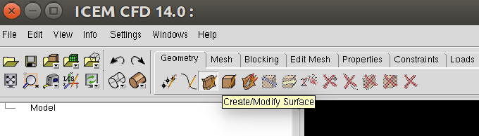
Under the Geometry tab, select Create/Modify Surface, as shown below:
A new menu will show up on the lower-left corner of the screen. Select Standard Shapes, then Box.
Finally, type ‘1 1 0’ in the X Y Z size field and click on ‘Apply’, just as shown below:
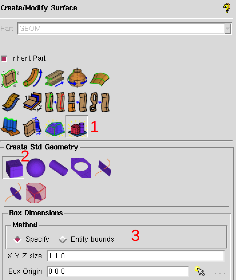
This function would usually generate the 6 surfaces of a box, but since we used Z size = 0, it will automatically give just a single surface in this case as the upper and lower sides of the box coincide.
Create parts for the edges
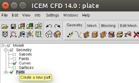
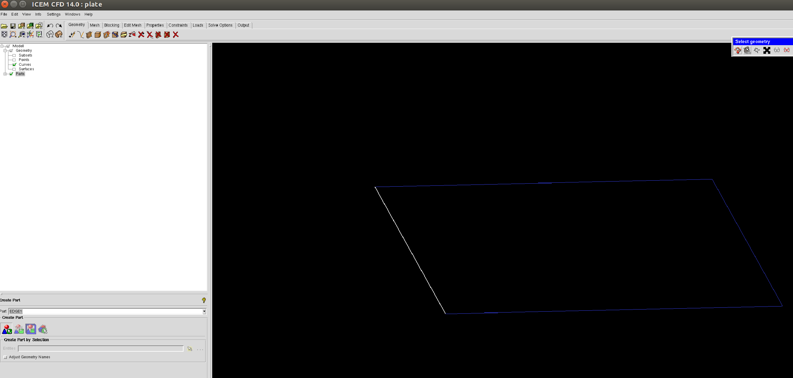
ICEM groups geometry components into Parts. We need to create Parts for the edges so that we can easily set up the boundary conditions later on. Look at the model tree on the left side of the screen and click with the right-mouse-button on the Parts branch. Select the Create Parts option. Also make sure that the Surfaces box in the Geometry branch in unchecked (otherwise it will be hard to select just the edges):
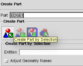
On the lower-left corner menu change the name of the part to ‘EDGE1’, then click on the Create Part by Selection, as shown below:
Click on one edge with the left-mouse-button in order to highlight it (see figure below) then click with the middle-mouse (scroll) button anywhere to confirm your selection. Now you can check if you have the EDGE1 component under the Parts branch in the model tree.
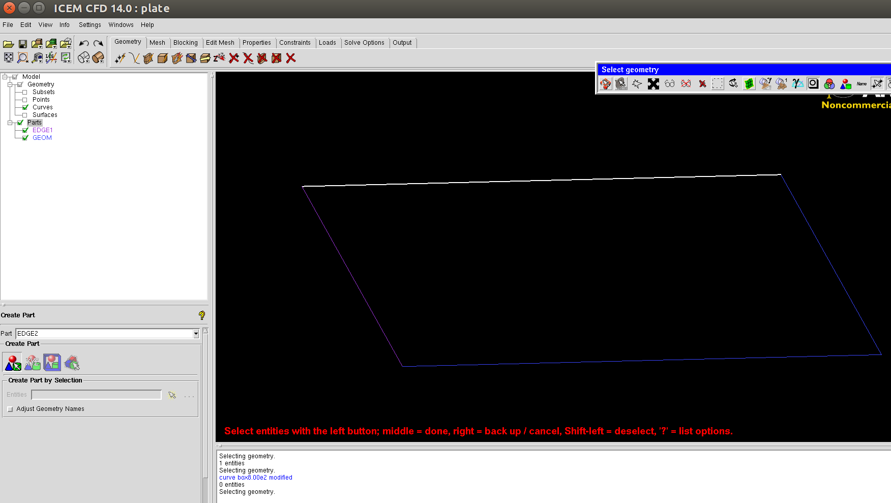
We can repeat the process to create the ‘EDGE2’ part. Remember to change the part name before selecting another edge. This time I chose the upper edge:
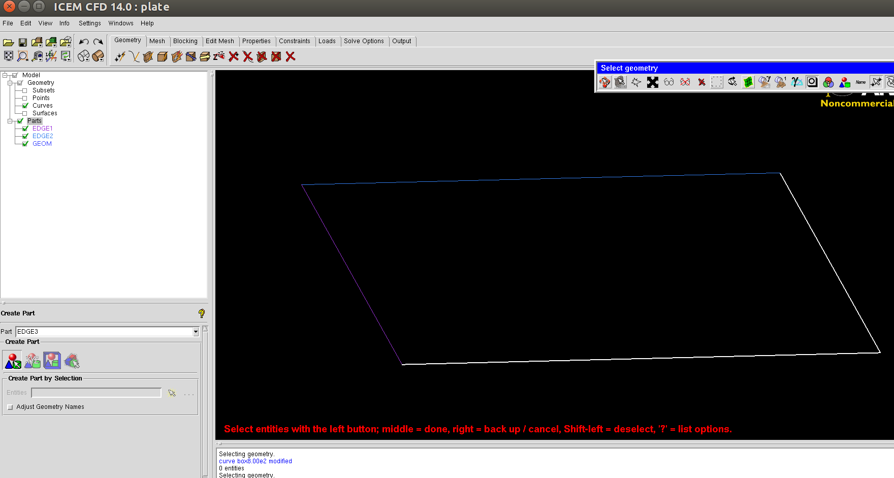
You can group multiple edges under the same Part if you want to apply the same boundary condition to all of them. For instance, we will create ‘EDGE3’ by grouping the remaining two edges. When selecting the edges, click on both of them with the left-mouse-button and only then you click with the middle-mouse-button to create the part.
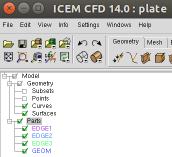
In the end, the Parts branch of the model tree should have three components: EDGE1, EDGE2, and EDGE3. Now you can also turn the Surface box back on. The model tree should look like this:
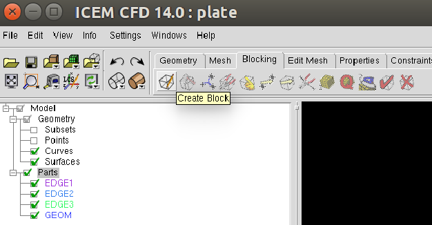
Create blocking
Now we need to create the blocks used by ICEM to generate meshes. Under the Blocking tab, choose Create Block:
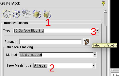
On the lower-left corner menu choose ‘2D Surface Blocking’ as Type, and select the ‘All Quad’ option under Free Mesh Type. Later, click on the Select surfaces(s) button:
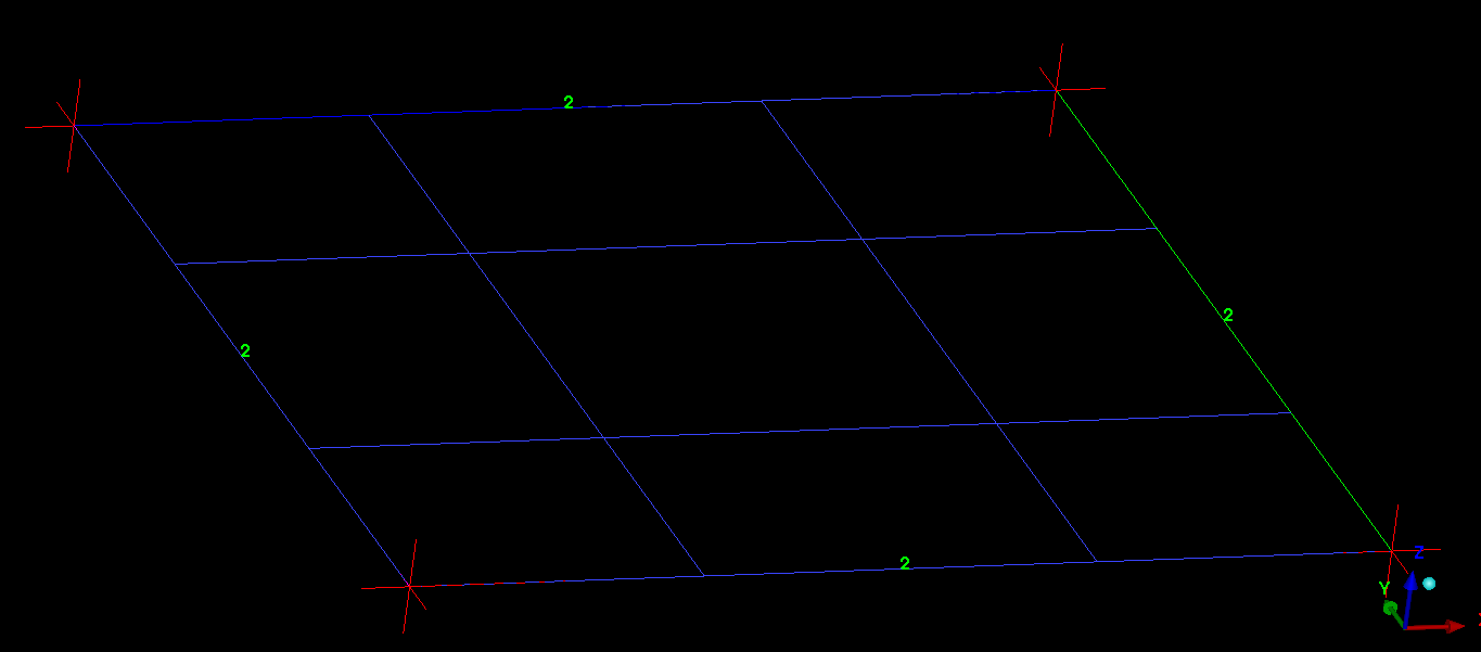
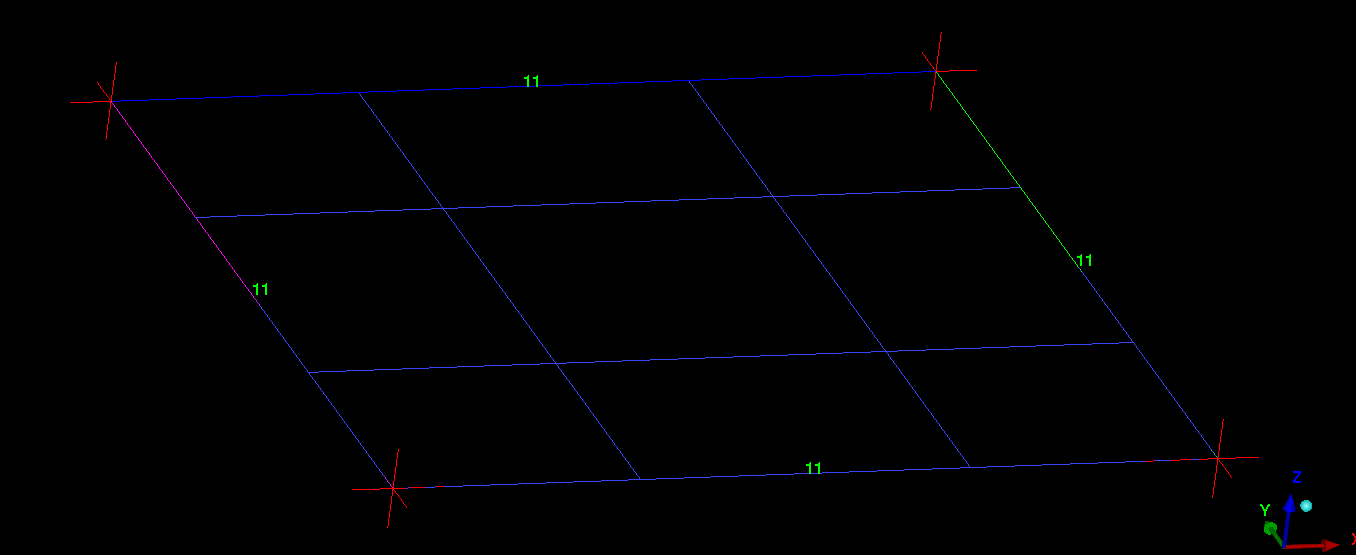
Now click on the flat square in order to highlight it (it should turn white), then click with the middle-mouse-button to confirm your selection. Finally, click on the Apply button to create the block (the square should turn back to blue). We can check if the blocking was done correctly by expanding the Blocking branch of the model tree. Click with the right-mouse-button on the Edges component and turn on the ‘Counts’ option. This will show how many nodes we have on each edge. For now, we should have two nodes per edge, as shown below:
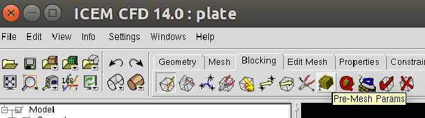
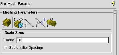
Let’s increase the number of nodes to make things more interesting. Under the Blocking tab, choose Pre-Mesh Params:
Select the Scale Sizes feature on the lower-left menu. Adjust the Factor option to 10 and click on Apply to globally refine the mesh:
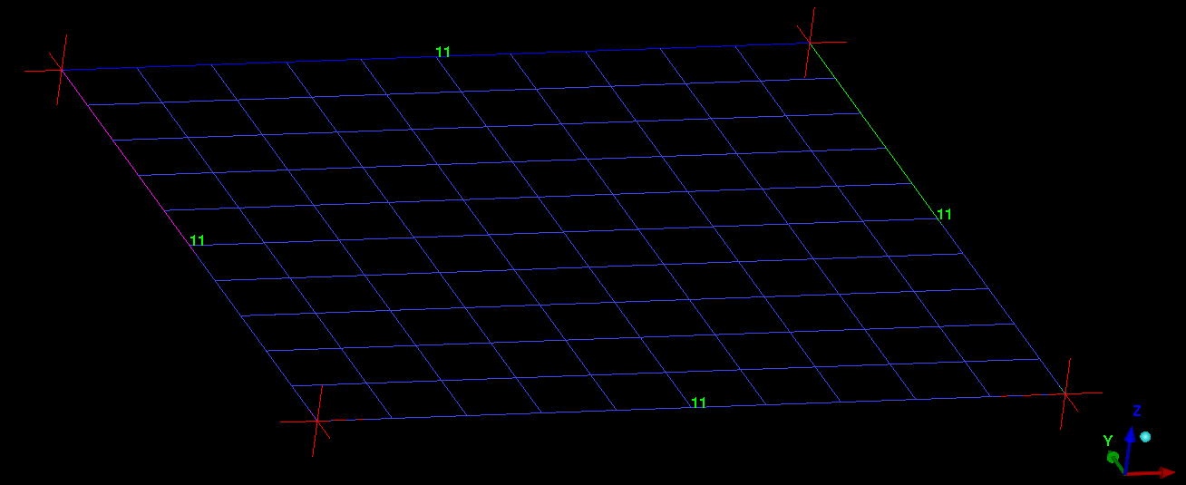
Now each edge should show 11 nodes:
Generate the Pre-mesh
It is time to generate the Pre-mesh. Just check the Pre-mesh box under the Blocking branch of the model tree and choose Yes. You should see all the surface cells now:
See if everything looks right in your Pre-mesh.
Preparing to export the mesh
Just to recap, we have done the following procedures:
Created our geometry in ICEM;
Created Parts grouping edges that will share same boundary conditions;
Added the surface blocks;
Generated the Pre-mesh.
Note
The procedures described from now on apply to any geometry. However, make sure you have followed all these steps above if you are working with your own geometry.
Now that we confirmed that the Pre-mesh looks right, we can generate the structured mesh. Click with the right-mouse-button on the Pre-mesh component under the Blocking branch of the model tree and choose Convert to MultiBlock Mesh. Save the project in the folder you just created. A new branch named Mesh should show up in your model tree.
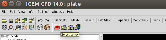
Next, we should select the export format. Under the Output folder, click on the Select Solver button (a red toolbox):
Choose the following options in the lower-left menu and click Apply:
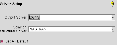
This will apply the CGNS format to our output. We will select the boundary conditions in the next step.
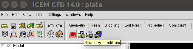
Applying boundary conditions
Under the Output folder, click on the Boundary condition button:
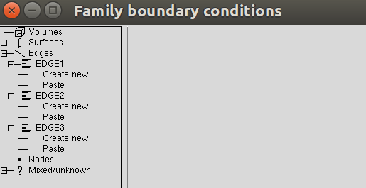
A new window should pop up. As we will apply boundary conditions (BCs) to the edges, expand everything under the Edges branch. You should see the edges Parts we defined previously (EDGE1, EDGE2, and EDGE3) as shown below. In some cases, they may end up under the Mixed/Unknown branch.
Symmetry plane
Let’s add a symmetry plane boundary condition to EDGE1. Click on the Create New branch under EDGE1. Another window will show up, where you should choose ‘BCType’ and click on ‘Okay’.
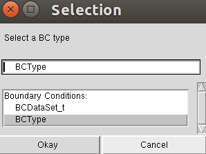
Now go back to the Boundary conditions window. If you click on the green button, you will see several types of Boundary Conditions. The currently supported types are:
BCExtrapolate -> Splay;
BCSymmetryPlane -> Symmetry X, Y, or Z planes;
BCWall -> Constant X, Y, or Z planes.
For this example, let’s choose ‘BCSymmetryPlane’ for this edge.
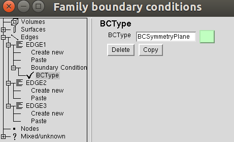
Now we need to specify if we want an X, Y, or Z symmetry plane. We will use a ‘Velocity’ node from the CGNS format in order to specify the reference plane. For instance, if we add a ‘VelocityX’ node to this boundary condition, we have a X symmetry plane, and the same for the other coordinates.
Do the following steps to add a X symmetry plane to the EDGE1 Part:
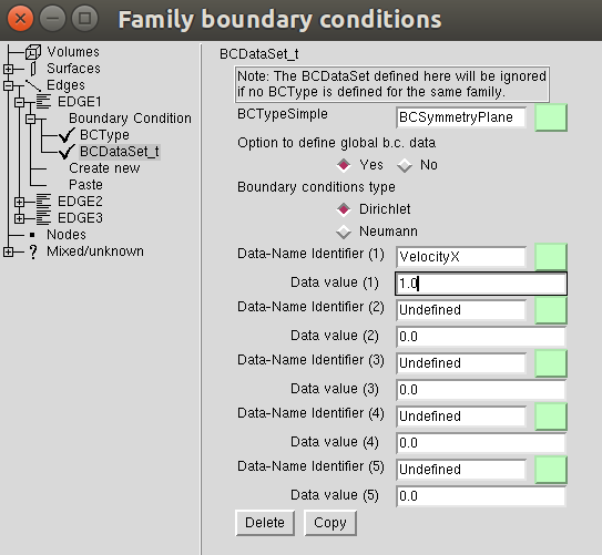
Click again on the Create New branch under EDGE1;
This time, select ‘BCDataset_t’ on the new window, and click on ‘Okay’;
Now back to the BC window, click on the green button near ‘BCTypeSimple’ and select ‘BCSymmetryPlane’;
Click on the green button that corresponds to the ‘Data-Name Identifier (1)’ field and choose ‘VelocityX’;
Change the ‘Data value (1)’ field to 1.0.
In the end, the options should look like the figure below:
In the case of a Y symmetry plane, you should select ‘VelocityY’ instead, and similarly for a Z symmetry plane. Do not click on Accept yet, otherwise it will close the window. Now let’s see the other edges.
Constant Plane
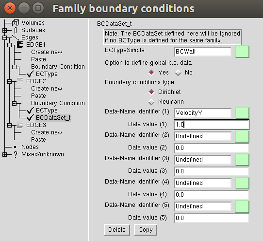
We will add a constant Y plane to EDGE2. Follow these steps:
Click on the Create New branch under EDGE2;
Select ‘BCType’ on the new window, and click on ‘Okay’;
Click on the green button of the BC window and select ‘BCWall’.
We still need to specify which coordinate (X, Y, or Z) should remain constant in this boundary condition. We will do this by adding a ‘Velocity’ option to this boundary condition.
Click again on the Create New branch under EDGE2;
This time, select ‘BCDataset_t’ on the new window, and click on ‘Okay’;
Now back to the BC window, click on the green button near ‘BCTypeSimple’ and select ‘BCWall’;
Click on the green button that corresponds to the ‘Data-Name Identifier (1)’ field and choose ‘VelocityY’;
Change the ‘Data value (1)’ field to 1.0.
In the end, the options should look like the figure below:
In the case of a constant X plane, you should select ‘VelocityX’ instead, and similarly for a constant Z plane. Do not click on Accept yet, because we still have one more boundary condition to go!
Splay
We’ll finally add a Splay boundary condition for the two edges included in the EDGE3 Part.
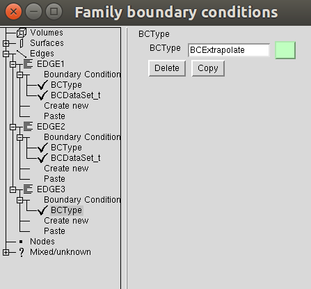
Click on the Create New branch under EDGE3;
Select ‘BCType’ on the new window, and click on ‘Okay’;
Click on the green button of the BC window and select ‘BCExtrapolate’.
This one was easier! The same BC will be applied to all edges in this Part. In the end, your boundary conditions tree should look like this:
Now we can click on Accept as we finished adding all the boundary conditions.
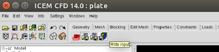
Exporting the mesh
We are ready to export the mesh! Click on the Write input button under the Output tab:
Save the project if asked for. Next we need to select the Multiblock mesh file. The name shown by default should be correct, so just click on ‘Open’. In the next window, click on ‘All’.
Another window with CGNS export options will show up. The default options should work fine, but you can compare it with the ones below. Make sure you are exporting a structured mesh:
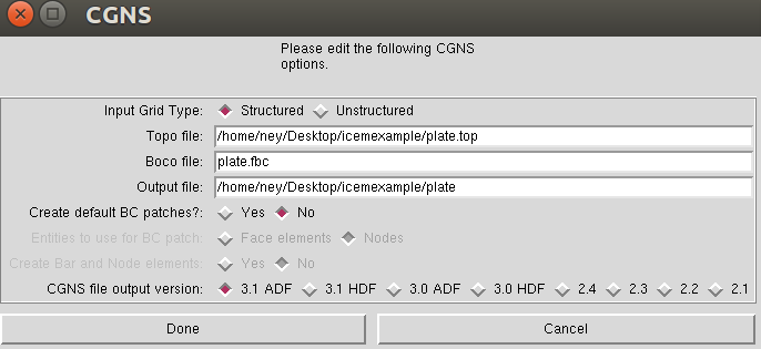
Click on ‘Done’ to finally conclude export procedure! A CGNS file should appear on your working folder. It will have the same name of the project file. This CGNS is ready to be used by pyHyp.
Checking the CGNS Structure
You can check if the CGNS file is correct by looking at its structure. If you have cgnslib installed, you can open the cgnsview GUI with the following command:
$ cgnsview
Open the newly generated CGNS file and expand its tree. For the flat square case, we have the following structure:
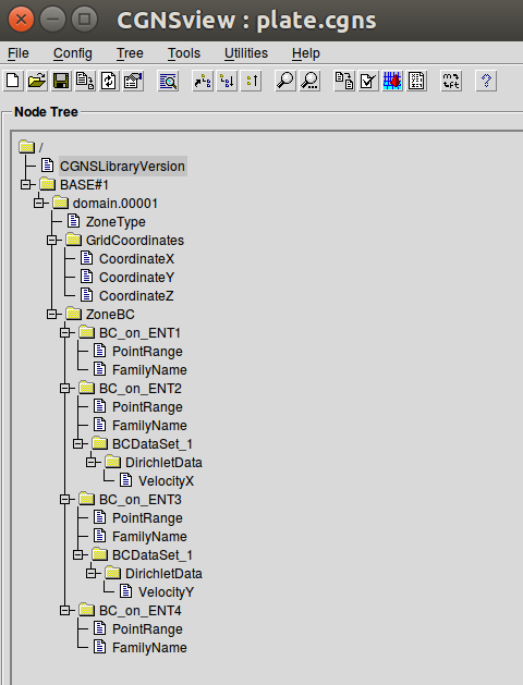
Note the VelocityX node indicating a X symmetry plane boundary condition and a VelocityY node indicating a constant Y plane boundary condition.
Boundary condition priorities
The corner nodes share two edges. Each edge may have different boundary conditions. The boundary condition at the corner node is chosen according to the following priority:
Constant X, Y, or Z planes
Symmetry X, Y, or Z planes
Splay
Therefore, if one edge that has a Splay BC is connected to another edge with a symmetry plane BC, the shared corner node will be computed with the symmetry plane BC.
Running pyHyp with the generated mesh
Create another empty folder and copy the CGNS file exported by ICEM to it. We can add the following Python script to the same folder:
from pyhyp import pyHyp

fileName = 'plate.cgns'
fileType = 'cgns'

options = {
    # ---------------------------
    #        Input File
    # ---------------------------
    'inputFile': fileName,
    'fileType': fileType,

    # ---------------------------
    #        Grid Parameters
    # ---------------------------
    'N': 65,
    's0': 1e-6,
    'marchDist': 2.5,

    # ---------------------------
    #   Pseudo Grid Parameters
    # ---------------------------
    'ps0': 1e-6,
    'pGridRatio': 1.15,
    'cMax': 5.0,

    # ---------------------------
    #   Smoothing parameters
    # ---------------------------
    'epsE': 1.0,
    'epsI': 2.0,
    'theta': 0.0,
    'volCoef': 0.3,
    'volBlend': 0.001,
    'volSmoothIter': 10,

    # ---------------------------
    #   Solution Parameters
    # ---------------------------
    'kspRelTol': 1e-15,
    'kspMaxIts': 1500,
    'kspSubspaceSize': 50,
    'writeMetrics': False,
    }


hyp = pyHyp(options=options)
hyp.run()
hyp.writeCGNS('plate3D.cgns')
Save this script with the name ‘generate_grid.py’. Then, navigate to the folder using the terminal and write the following command:
$ python generate_grid.py
This script will read the plate.cgns file (which contains the surface mesh and the boundary conditions) and will generate the plate3D.cgns file with the volume mesh. It is important to check the ‘MinQuality’ column of the screen output. A valid mesh should have only positive values.
You can also run pyHyp in parallel with the following command:
$ mpirun -np 4 python generate_grid.py
The option ‘-np 4’ indicates that 4 processors will be used. The results may vary slight due to the parallel solution of the linear system.
Visualizing the mesh in TecPlot 360
If you have TecPlot 360 installed in your computer you can visualize the volume mesh. Open a terminal and navigate to the folder than contains the newly generated CGNS file with the volume mesh. Then type the following command:
$ tec360
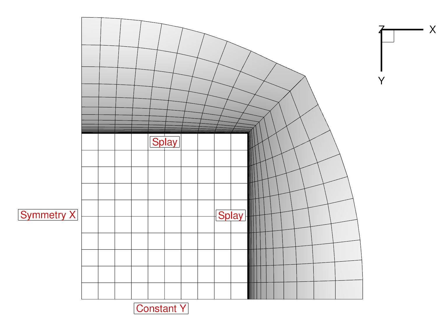
This will open TecPlot 360. On the upper menu select ‘File’ > ‘Load Data Files’, then choose your CGNS file. Next, check the ‘Mesh’ box on the left panel, and click ‘Yes’. You will be able to visualize the mesh as shown below:
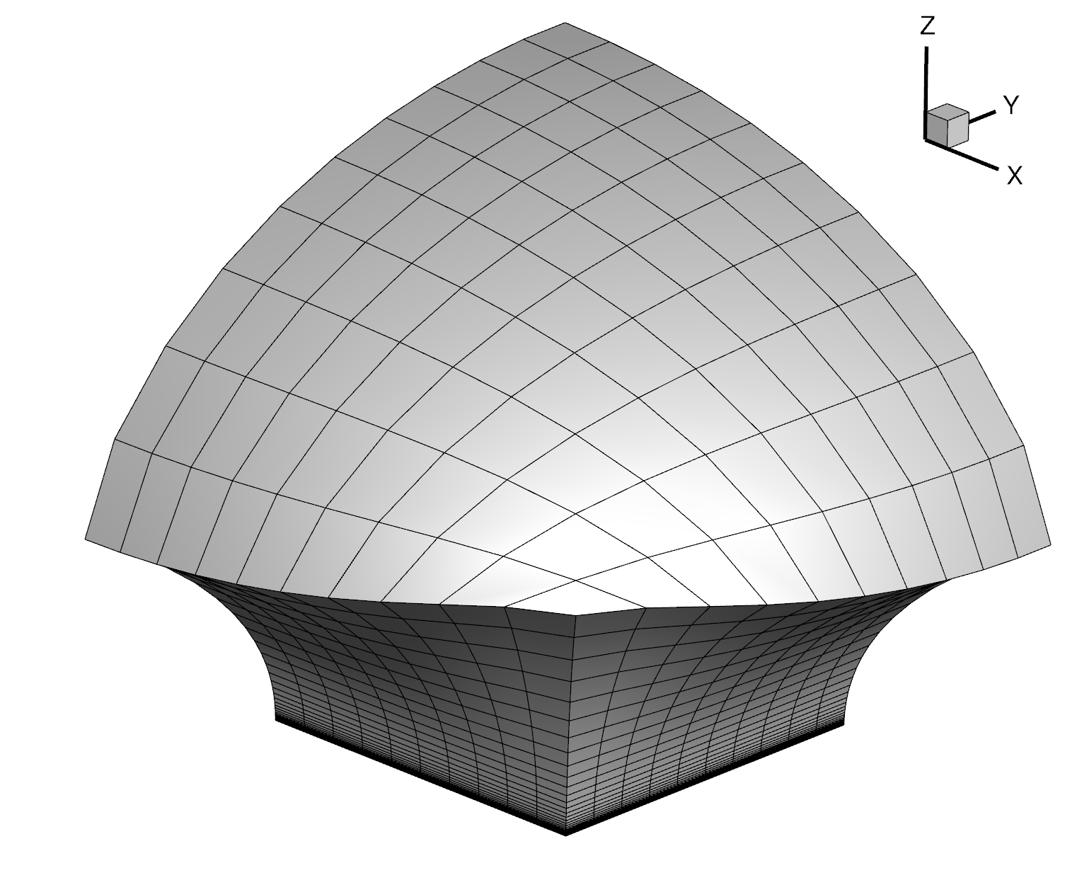
We can see that the boundary conditions where correctly applied. The image below shows a bottom view of the mesh:
Try playing with the different parameters to see their impact on the final mesh. In this case, it is helpful to save a TecPlot layout file. For instance, place the mesh in a position you want and click on ‘File’ > ‘Save Layout File’ and save it with the name you want (let’s say layout_hyp.lay). Then you can open you mesh directly from the command line by typing:
$ tec360 layout_hyp.lay
Then you don’t have to go over the menus all over again!