Tips for Coarse Grids
Generating very coarse meshes for adaptive runs can be challenging with pyHyp. This page discusses a few tips and tricks to keep in mind when trying to make starting meshes for adaptive runs. Most of this information assumes that the final grid is independent of the starting grid. This means that most of these tips are given with the intent of getting the first grid to converge any sort of solution that will allow the adaptive meshing algorithm to take over. The coarser the initial mesh, the more work the adaptive algorithm can do, hopefully reducing the discretization error as much as possible.
The obvious way to do this is to generate a typical mesh and then call cgns_utils coarsen to coarsen the grid to the desired level.
This method does work, but it doesn’t provide the user with obvious ways to make quick changes to a grid.
As an example, how do we ensure that a grid will have an initial off wall spacing of a certain value after a number of calls to cgns_utils?
The answer is too much math and thinking, and it would unnecessarily add some number of cgns_utils coarsen calls to the workflow.
Suffice to say it would be much easier to make a grid where the initial output is of interest rather than the output after a number of calls to cgns_utils.
With that in mind, this discussion will provide methods for getting a coarse grid straight out of pyHyp.
This discussion will use a 2D RAE 2822 airfoil as an example. Even though this is restricted to a rather simple 2D case, the tips can be extended to 3D and more complex geometries. Below is an example of a mesh that pyHyp created with obvious negative volumes. This is a bit of a ridiculous example, but someone actually managed to get a grid that looked like this on accident.
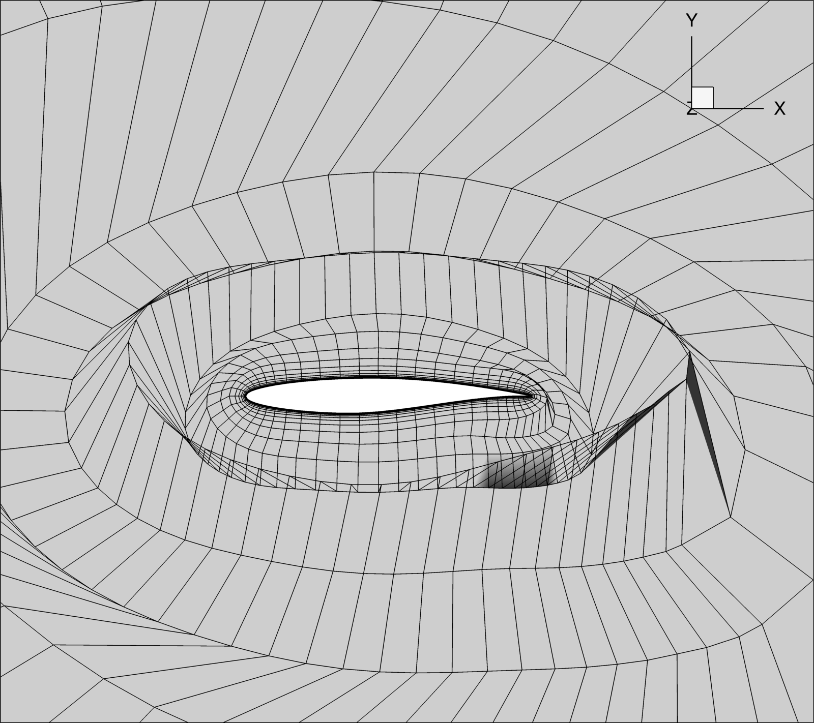
This grid was created using a surface mesh with 50 points around the airfoil and the following non-default options:
options = {
    # ---------------------------
    #        Input Parameters
    # ---------------------------
    "inputFile": "rae2822.xyz",
    "unattachedEdgesAreSymmetry": False,
    "outerFaceBC": "farfield",
    "autoConnect": True,
    "BC": {
        1: {
            "jLow": "zSymm",
            "jHigh": "zSymm",
        }
    },
    "families": "wall",
    # ---------------------------
    #        Grid Parameters
    # ---------------------------
    "N": 31,
    "s0": 4e-5,
    "marchDist": 100.0,
    "nConstantStart": 1,
    # ---------------------------
    #   Pseudo Grid Parameters
    # ---------------------------
    "cMax": 3.0,
}
There are a few ways to try and fix this problem with the grid.
The first thing to check is to make sure that cMax is set to 1.
cMax can be increased if the geometry is simple enough to speed up grid generation by sacrificing robustness.
Whenever a grid is having trouble converging, always try decreasing cMax first.
Even if this removes all the negative volumes, it may still result in some undesirable twist in the cells in the grid.
This twist should be okay if the adaptive algorithm regenerates a grid at each step since it will disappear when the next grid is generated.
However, if the adaptive algorithm splits cells that already exist, then it may be prudent to try to remove cells that are twisted to avoid skewed cells during adaptation.
One possible fix is to increase N, the number of steps to reach the march distance.
This allows pyHyp to take more gradual steps, meaning it is less likely to twist the grid into weird shapes.
Those first two tips will normally fix any obvious problems in the grid.
Sometimes there may still be extremely skewed cells close to the airfoil, which sometimes can result in small negative volumes near the trailing edge.
A key point to remember about this initial grid is that only a converged solution is needed, not a good one.
In a typical grid, the initial grid spacing, s0, needs to be set to a certain amount based off a desired y+ value.
To handle these skewed cells, more points around the airfoil would need to be sampled to retain the desired s0, but in this case more grid points are undesirable.
In adaptive meshing, the algorithm is expected to determine what “value” of s0 is needed.
Therefore, s0 should be increased to whatever the flow solver can converge and then the algorithm will worry about the initial grid spacing.
In this case, s0 could be increased to 1e-3 before the flow solver had trouble.
This process can be trial and error, and with grids this coarse, it should not be too much trouble.
The next image shows a grid that pyHyp generated with the same surface mesh after modifying some of the options.
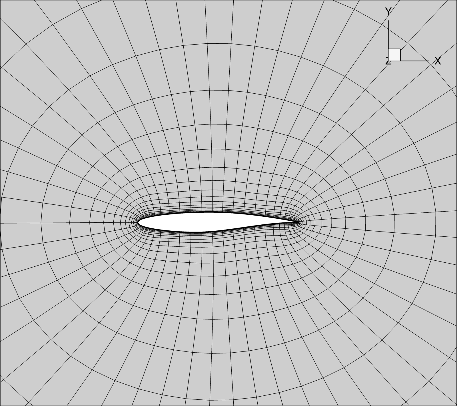
Much better!
options = {
    # ---------------------------
    #        Input Parameters
    # ---------------------------
    "inputFile": "rae2822.xyz",
    "unattachedEdgesAreSymmetry": False,
    "outerFaceBC": "farfield",
    "autoConnect": True,
    "BC": {
        1: {
            "jLow": "zSymm",
            "jHigh": "zSymm",
        }
    },
    "families": "wall",
    # ---------------------------
    #        Grid Parameters
    # ---------------------------
    "N": 31,
    "s0": 1e-3,
    "marchDist": 100.0,
    "nConstantStart": 1,
    # ---------------------------
    #   Pseudo Grid Parameters
    # ---------------------------
    "cMax": 1.0,
}